Valentius Kryptix

Introduction

Machine learning is a branch of artificial intelligence that enables computers to identify patterns in data and make predictions without explicitly programming every decision. One of the most fundamental machine learning algorithms is linear regression, which predicts continuous numerical values using relationships between input features and a target variable.

As part of my ML Fundamentals internship project at Valentius Kryptix, I implemented linear regression entirely from scratch using Python and NumPy. Instead of relying on ready-made machine learning models, I developed the prediction function, cost function, and gradient descent optimization algorithm manually.

The main objective was to understand what happens internally when a linear regression model learns from data.

Understanding Linear Regression

Linear regression is a supervised learning algorithm used to predict numerical values.

For example, it can be used to predict house prices based on median income, house age, population, and other characteristics.

In simple linear regression, the relationship between an input feature and the predicted output can be represented as:

ŷ = θ₀ + θ₁x

Here, θ₀ represents the intercept, θ₁ represents the coefficient, and x represents the input feature.

Multiple linear regression extends this equation by incorporating several input features.

ŷ = θ₀ + θ₁x₁ + θ₂x₂ + … + θₙxₙ

In my project, I implemented both approaches using NumPy matrix operations.

Project Objective

The primary objective of this project was to build a linear regression model without using a prebuilt regression algorithm.

The implementation focused on understanding how predictions are generated, how prediction errors are calculated, and how model parameters are optimized through gradient descent.

Scikit-learn was used only for dataset splitting and final comparison with the custom regression implementation.

California Housing Dataset

I used the California Housing dataset, which contains 20,640 housing records.

The dataset includes eight input features:

• Median income
• Median house age
• Average rooms per household
• Average bedrooms per household
• Population
• Average occupancy
• Latitude
• Longitude

The target variable, MedHouseVal, represents the median house value in units of $100,000.

For simple linear regression, I selected median income as the input feature. For multiple linear regression, I used all eight features.

Data Preprocessing

Before training the model, I explored the dataset using Pandas and checked for missing values.

The dataset was divided into 80% training data and 20% testing data.

This resulted in 16,512 training records and 4,128 testing records.

I also standardized the input features using NumPy.

X_scaled = (X − μ) / σ

Standardization transforms features so they have approximately zero mean and unit standard deviation.

This step was important because the housing dataset contains features with different numerical ranges. Standardization helped gradient descent optimize the model parameters more efficiently.

To avoid data leakage, the mean and standard deviation were calculated using only the training data.

Implementing Linear Regression From Scratch

The implementation involved three major mathematical components.

1. Hypothesis Function

The hypothesis function generates predictions using the input features and model parameters.

h(X) = Xθ

I implemented this using NumPy matrix multiplication.

The model parameters were initially set to zero. During training, gradient descent updated these parameters to reduce prediction errors.

2. Mean Squared Error Cost Function

To measure prediction errors, I implemented the Mean Squared Error (MSE) cost function.

MSE = (1/m) Σ(ŷᵢ − yᵢ)²

This calculates the average squared difference between predicted and actual values.

A lower MSE indicates smaller prediction errors.

The cost function helped measure whether the model was improving during training.

3. Gradient Descent Optimization

Gradient descent is an optimization algorithm that iteratively adjusts model parameters to minimize the cost function.

The update rule is:

θ = θ − α∇J(θ)

Here, α represents the learning rate, which controls the size of each parameter update.

For the MSE cost function, the gradient is:

∇J(θ) = (2/m)Xᵀ(Xθ − y)

I implemented the gradient calculations and parameter updates manually using NumPy.

For multiple regression, I used a learning rate of 0.01 and trained the model for 10,000 iterations.

The training cost decreased significantly, demonstrating that gradient descent was successfully optimizing the model parameters.

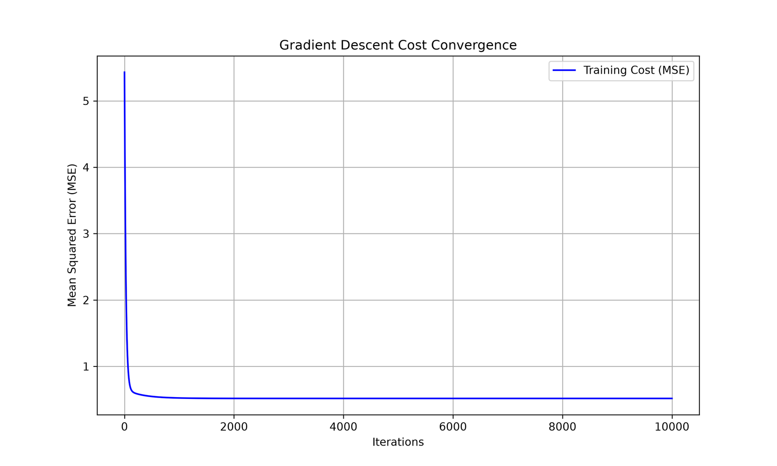
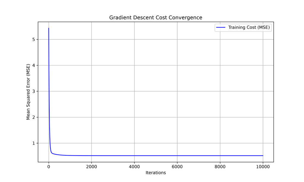
Visualizing Gradient Descent Convergence

An important part of the project was visualizing how the cost function changed during training.

I recorded the MSE after each gradient descent iteration and plotted the results using Matplotlib.

The graph showed a downward trend, indicating that the model’s prediction errors decreased as training progressed.

For multiple linear regression, the initial training MSE was approximately 5.6297 and decreased substantially during optimization.

Insert the cost convergence graph here.

Model Evaluation and Results

After training, I evaluated both regression models using unseen testing data.

I manually calculated Mean Squared Error and the R² score using NumPy rather than relying on predefined evaluation functions.

The simple linear regression model achieved:

• Testing MSE: 0.709116
• Testing R²: 0.458859

The multiple linear regression model achieved approximately:

• Testing MSE: 0.556
• Testing R²: 0.576

The multiple regression model performed better because it incorporated additional housing features.

The R² score indicates how much of the variation in the target values is explained by the model relative to predicting the mean.

Comparison With Scikit-Learn

To verify my implementation, I compared the custom NumPy model against scikit-learn’s LinearRegression.

Both models were trained using the same training dataset and evaluated using the same testing dataset.

Initially, some coefficients differed because gradient descent had not fully converged.

After increasing the number of training iterations to 10,000, the results became extremely close.

The mean absolute prediction difference between the two implementations was approximately 0.00000618.

This provided strong evidence that the custom gradient descent implementation was functioning correctly.

Key Learnings

This project helped me understand several fundamental machine learning concepts.

First, I gained practical experience implementing mathematical equations using NumPy arrays and matrix operations.

Second, I learned how learning rates, feature standardization, and training iterations affect gradient descent convergence.

Third, I understood why evaluating a model on unseen data is essential for measuring its predictive performance.

Finally, comparing the custom implementation with scikit-learn demonstrated the importance of validating machine learning algorithms.

Conclusion

Building linear regression from scratch was a valuable learning experience that strengthened my understanding of machine learning fundamentals.

Rather than treating machine learning libraries as black boxes, this project helped me understand how predictions, errors, gradients, and parameter updates work together.

The multiple regression model achieved better predictive performance than the simple regression model, while the comparison with scikit-learn confirmed that the custom implementation produced nearly identical predictions.

This project provides a foundation for exploring more advanced machine learning algorithms and optimization techniques.

GitHub Repository: https://github.com/psarya/Linear-Regression-From-Scratch