Valentius Kryptix

Introduction

Most of the data in the real world doesn’t come with answers attached. Nobody hands you a column saying which customer is “loyal” or which product is “premium.” Unsupervised learning is the branch of machine learning that finds patterns in data without being told what to look for.

During my internship at Valentius Kryptix, I built an unsupervised learning pipeline using K-Means clustering and Principal Component Analysis (PCA). I ran it on the Wine dataset, which has 178 wines described by 13 chemical measurements such as alcohol, flavanoids, color intensity and proline. The dataset includes the grape cultivar for each wine, but I hid it while clustering. I used it only afterwards, as a check on whether the algorithm had found something real.

Step 1: Scaling the data

K-Means groups points by distance, so features measured on larger scales dominate the result. In this dataset, proline ranges from roughly 280 to 1,680, while hue sits between about 0.5 and 1.7. Without scaling, proline alone would decide almost every cluster assignment.

I used StandardScaler to give every feature a mean of 0 and a standard deviation of 1, so each chemical property counted equally.

Step 2: Choosing k instead of guessing

K-Means needs you to pick the number of clusters in advance, and choosing badly gives meaningless results. I tested k from 2 to 10 using two methods:

• The elbow method plots inertia, the total squared distance from points to their cluster centers. Inertia always falls as k rises, so you look for the point where the improvement slows. It dropped by about 381 from k=2 to k=3, but only about 103 from k=3 to k=4. The bend is at k=3.
• The silhouette score measures how well each point fits its own cluster compared with the nearest other one. It peaked at k=3 with a score of 0.285.

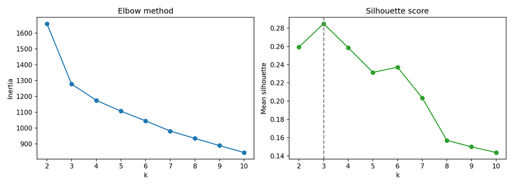
Two independent methods agreeing gave me real confidence in k=3. A silhouette of 0.285 is moderate. It says the groups are real but not sharply separated, which is normal for real data.

Step 3: Seeing 13 dimensions with PCA

Nobody can plot 13 dimensions, so I used PCA to project the scaled data down to two. PCA finds the directions along which the data varies most and ranks them.

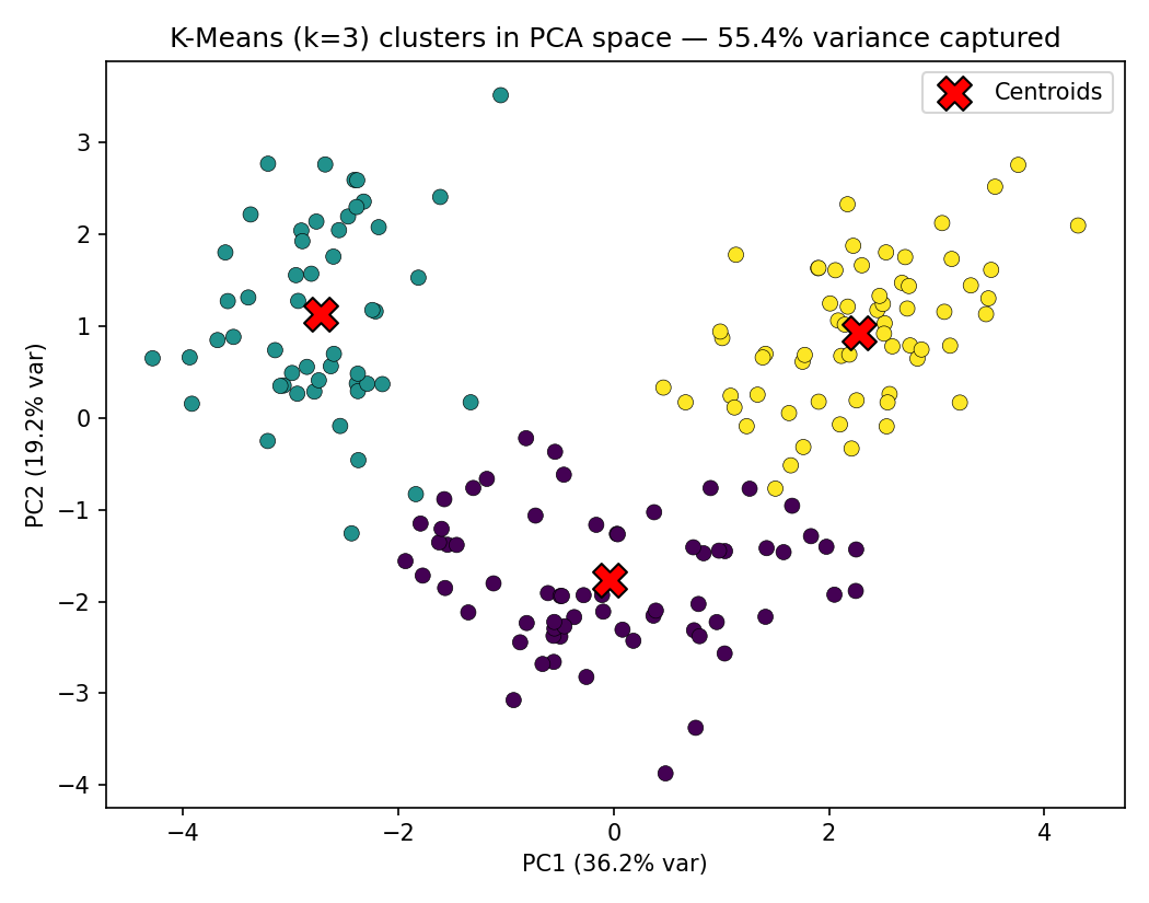
The first component explained 36.2% of the variance and the second explained 19.2%. Together, my 2D plot captures 55.4% of the original information.

That number matters. It means the plot is a helpful picture but not the whole story, and clusters that overlap on screen may be separate in the full 13-dimensional space. An important detail is that I ran K-Means on the full scaled data and used PCA only to visualize the result, so the clustering never depended on the projection.

Step 4: What do the clusters mean?

Clustering is only useful if you can explain the groups. I compared the average feature values of each cluster:

• Cluster 2 (62 wines): full-bodied and phenolic-rich. It has the highest proline (about 1,100), the most flavanoids, and the highest alcohol (about 13.7).
• Cluster 1 (51 wines): dark but low in phenolics. Its color intensity is very high (about 7.2) and so is its malic acid, but it has the lowest flavanoids and hue.
• Cluster 0 (65 wines): light and low-alcohol. It has the lowest alcohol (about 12.3) and the palest color, with low proline.

To test the result, I compared the clusters with the hidden cultivar labels. The Adjusted Rand Index was 0.897, and only about 6 of the 178 wines landed in a different group from their true cultivar. The algorithm recovered the three grape varieties using chemistry alone, with no labels.

What I learned

1. Preprocessing decides the outcome. Skipping scaling would have produced clusters driven by one feature.
2. Validate your choices with more than one method. The elbow and the silhouette score each have weaknesses, and agreement between them is more trustworthy than either alone.
3. Be honest about what a visualization shows. Reporting the explained variance ratio keeps you from over-reading a 2D plot.
4. Interpretation is the real deliverable. Cluster numbers mean nothing until you translate them into something a person can understand.

Limitations

K-Means assumes roughly round, similarly sized clusters, and it can struggle with irregular shapes. My dataset is also small, at 178 samples. I fixed the random seed and used 20 initializations to keep the results stable. For a larger project I would try Gaussian Mixture Models or DBSCAN and compare them with K-Means.

Conclusion

This project showed me that unsupervised learning is as much about judgment as algorithms: how you prepare the data, how you justify k, and how you explain the result. The full code, plots and write-up are on GitHub: https://github.com/VivekChaudhari786/K-means-Cluster-and-PCA

Thank you to Valentius Kryptix for the opportunity to work on this.