Valentius Kryptix

Introduction

Machine Learning is an important field of Artificial Intelligence that enables computers to learn patterns from data and make predictions without being explicitly programmed for every situation. Understanding the fundamentals of Machine Learning is essential for developing reliable and effective predictive models.

As part of my internship task at Valentius Kryptix, I worked on an ML Fundamentals project focused on implementing a Linear Regression model from scratch using NumPy. The main objective of this project was to understand the mathematical concepts and optimization process behind Linear Regression rather than simply using a ready-made Machine Learning library.

This project helped me understand how data is prepared, how predictions are generated, how errors are measured, and how model parameters are updated during training.

What is Linear Regression?

Linear Regression is a supervised Machine Learning algorithm used to predict a continuous numerical target variable based on one or more input features.

For example, Linear Regression can be used for applications such as:

• House price prediction
• Salary prediction
• Sales forecasting
• Demand prediction
• Temperature prediction

In multiple Linear Regression, the prediction can be represented using the equation:

h(X) = Xθ

Here, X represents the input feature matrix and θ represents the model parameters or coefficients.

The main objective is to find the best values of the parameters so that the predicted values are as close as possible to the actual target values.

Dataset Used

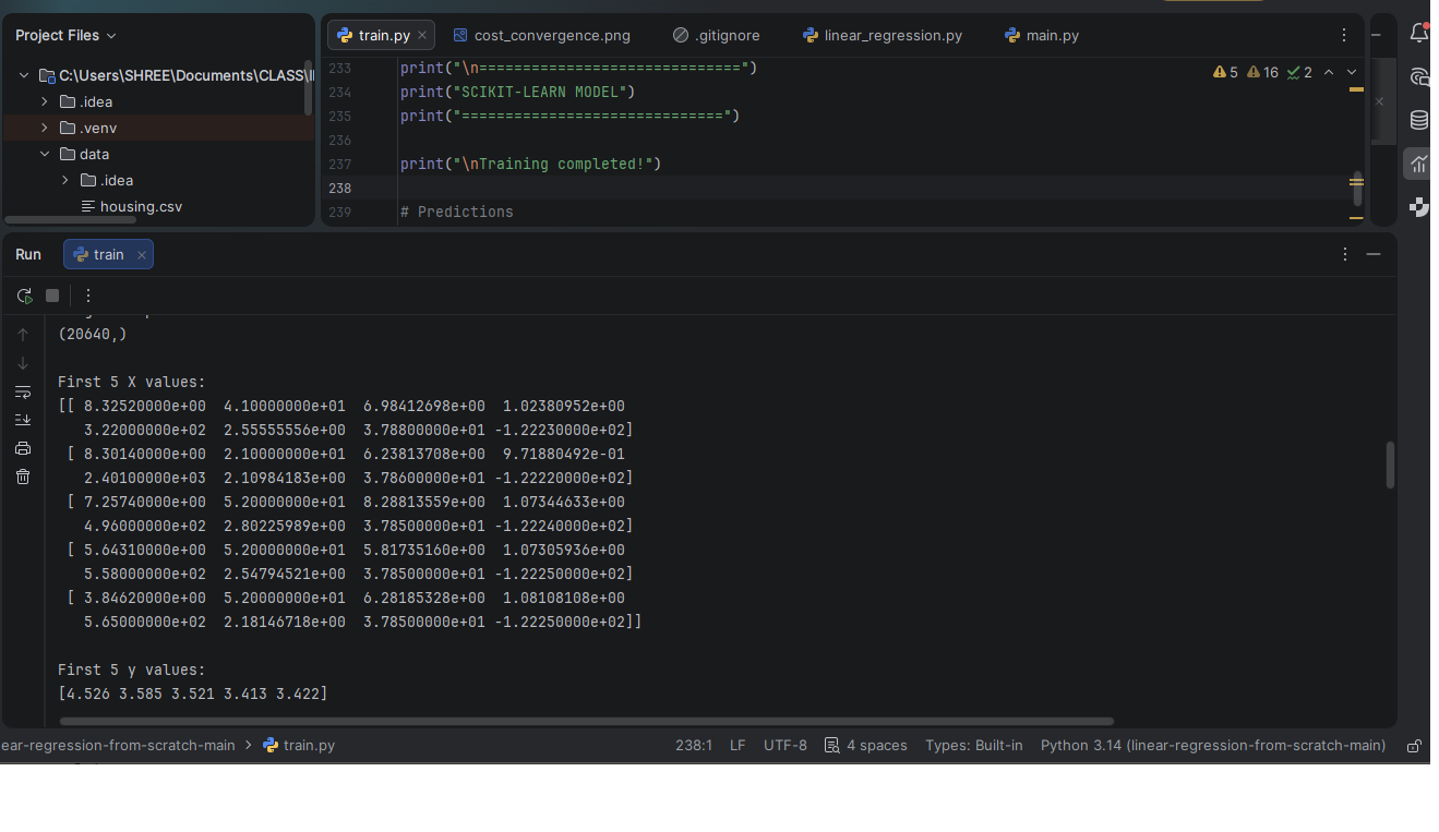
For this project, I used the California Housing dataset. It is a real-world dataset containing information about housing characteristics and house values.

The dataset contains multiple numerical features, including information related to:

• Median income
• House age
• Average number of rooms
• Average number of bedrooms
• Population
• Average occupancy
• Latitude
• Longitude

The target variable represents the median house value.

Train-Test Split

To evaluate the model properly, the dataset was divided into training and testing sets.

The training dataset was used to learn the model parameters, while the testing dataset was kept separate and used only for final evaluation.

In my implementation, the dataset was divided into approximately:

• 80% Training Data
• 20% Testing Data

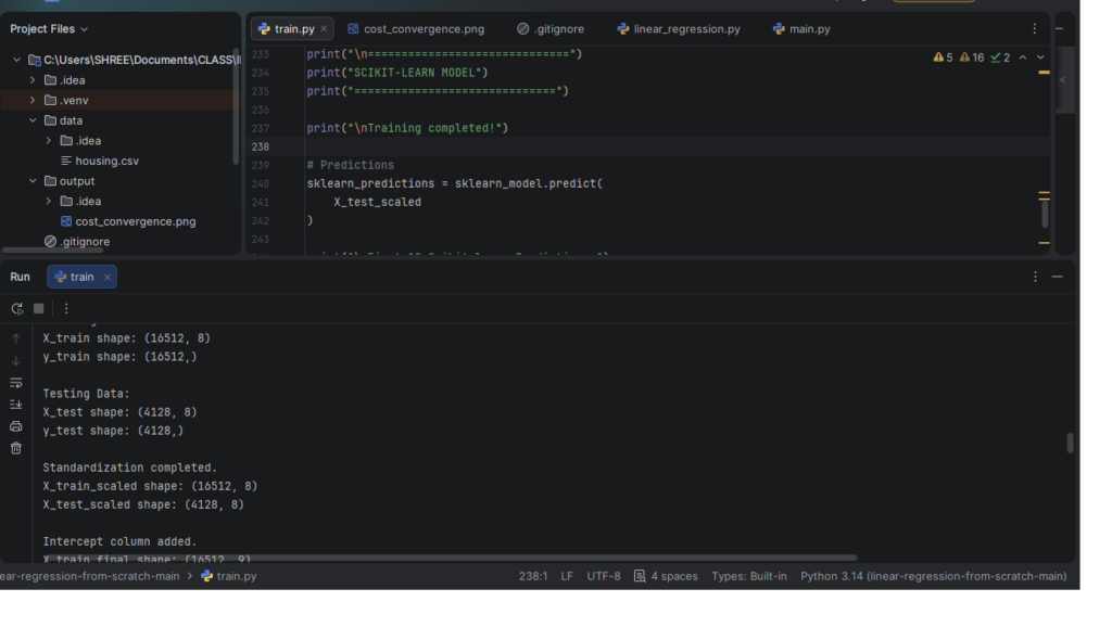
The resulting shapes were:

X_train shape: (16512, 8)
y_train shape: (16512,)

X_test shape: (4128, 8)
y_test shape: (4128,)

This separation helps evaluate how well the model performs on data that it has not seen during training.

Feature Standardization

The input features have different numerical ranges. For example, income, population, house age, and geographical values can have very different scales.

To improve the performance and stability of Gradient Descent, I standardized the input features.

The standardization formula is:

X_scaled = (X – mean) / standard deviation

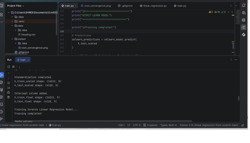
The mean and standard deviation were calculated using the training data. The same values were then applied to the testing data.

After standardization, the feature values were placed on a comparable scale.

X_train_scaled shape: (16512, 8)
X_test_scaled shape: (4128, 8)

Hypothesis Function

The first important component of the Linear Regression model is the hypothesis function.

The hypothesis function generates predictions from the input features and model parameters.

The mathematical representation is:

h(X) = Xθ

I implemented this operation using NumPy matrix multiplication:

def hypothesis(self, X):
return np.dot(X, self.theta)

Using NumPy’s dot() operation allows the model to perform the matrix multiplication efficiently without relying on a ready-made regression algorithm.

Mean Squared Error Cost Function

The model needs a way to measure how far its predictions are from the actual target values.

For this purpose, I implemented the Mean Squared Error based cost function.

The cost function used in the implementation is:

J(θ) = 1/(2m) Σ(prediction – actual)²

Here:

• m represents the number of training examples.
• Prediction represents the value generated by the model.
• Actual represents the true target value.

The errors are squared so that positive and negative errors do not cancel each other out.

A lower cost means that the predictions are closer to the actual values.

Gradient Calculation

After calculating the cost, the model needs to determine how the parameters should be changed.

For this purpose, I implemented the gradient of the cost function.

The gradient formula is:

∇J(θ) = 1/m Xᵀ(Xθ – y)

The implementation uses NumPy matrix operations:

gradient = (1 / m) * np.dot(X.T, errors)

The gradient indicates the direction in which the cost function changes with respect to the model parameters.

Gradient Descent

Gradient Descent is the optimization algorithm used to train the model.

The parameter update rule is:

θ = θ – α × gradient

where:

• θ = model parameters
• α = learning rate
• gradient = gradient of the cost function

During each iteration, the model calculates the gradient and updates the parameters.

The process is repeated for multiple iterations until the cost function gradually decreases and the model reaches a suitable solution.

The training loop was implemented manually using NumPy.

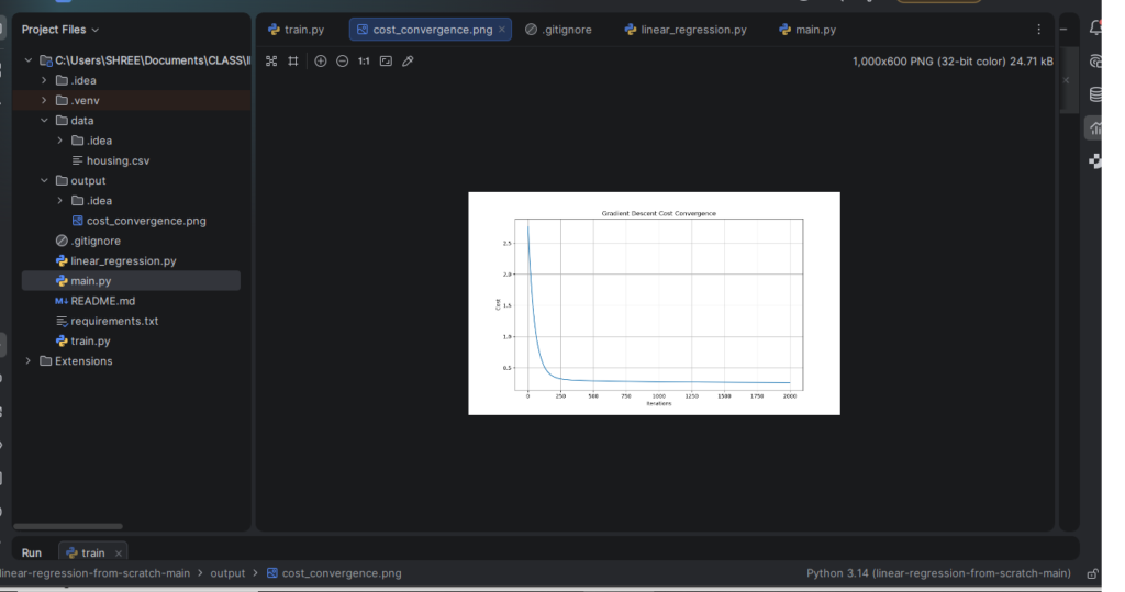
Cost Function Convergence

To verify that Gradient Descent was actually learning, I stored the cost value after every training iteration.

The stored cost values were then plotted using Matplotlib.

A successful training process should show a decreasing cost curve. This indicates that the model is gradually reducing its prediction error.

[ADD YOUR COST CONVERGENCE GRAPH HERE]

Figure 4: Cost function decreasing during Gradient Descent training.

This graph provides a visual representation of the optimization process and helps identify whether the selected learning rate is appropriate.

Model Evaluation

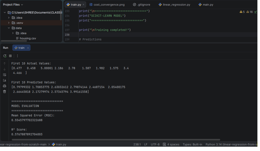
After completing the training process, I used the trained model to generate predictions on the test dataset.

The model was evaluated using two important metrics:

Mean Squared Error

Mean Squared Error measures the average squared difference between predicted and actual values.

A lower MSE generally indicates that the predictions are closer to the actual values.

R² Score

R², or the coefficient of determination, measures how well the model explains the variation in the target variable.

An R² value closer to 1 generally indicates that the model explains a larger proportion of the variation in the target variable.

For this project, both MSE and R² were calculated manually rather than using a ready-made evaluation function.

Comparison with Scikit-Learn

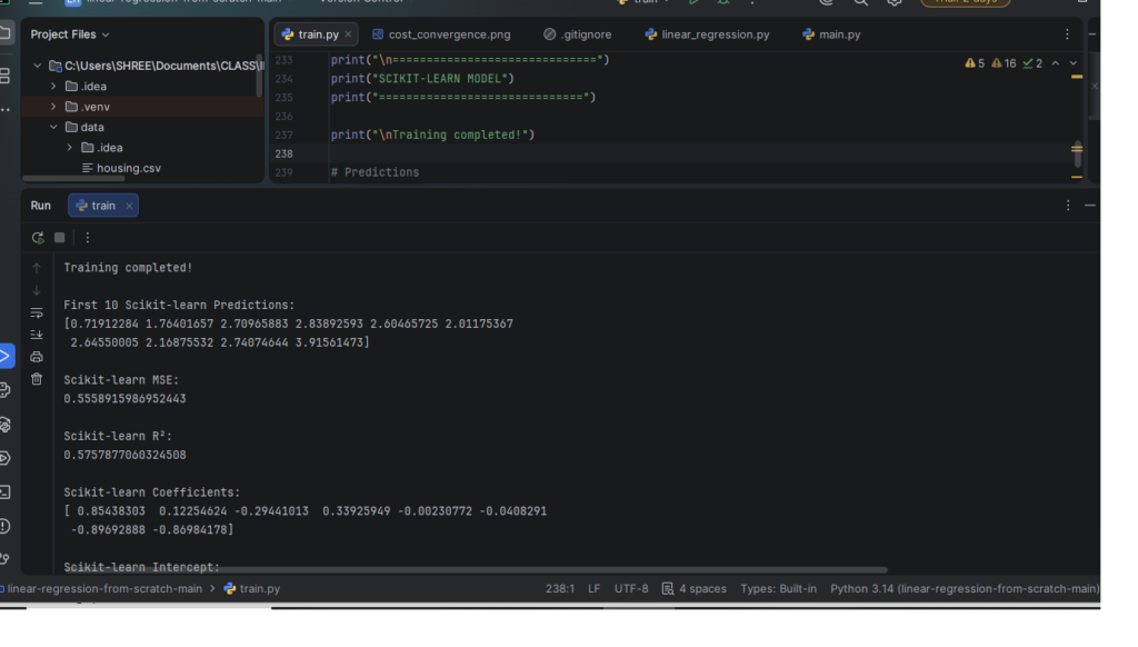
After implementing Linear Regression completely from scratch, I compared the custom implementation with the LinearRegression model available in Scikit-Learn.

The same training and testing datasets were used for both models.

The comparison included:

• Model coefficients
• Predictions
• Test MSE
• R² score

The purpose of this comparison was to verify the correctness of the manually implemented mathematical operations.

The scratch implementation should produce results that are reasonably close to the Scikit-Learn implementation when the same preprocessing and data split are used.

Tools and Technologies Used

The following technologies and libraries were used in this project:

Python — Main programming language.

NumPy — Used for mathematical operations, arrays, matrix multiplication, cost calculation, gradients, and parameter updates.

Pandas — Used for loading and processing the dataset.

Matplotlib — Used to visualize the cost convergence during training.

Scikit-Learn — Used only for the final comparison and sanity check, not for implementing the main Linear Regression model.

PyCharm — Used as the development environment for writing and running the Python code.

What I Learned

This project helped me develop a stronger understanding of Machine Learning fundamentals.

I learned how a Linear Regression model generates predictions using matrix multiplication and how the cost function measures prediction errors.

I also learned how Gradient Descent works internally and how the learning rate affects the optimization process.

Other important concepts I practiced include:

• Data preprocessing
• Train-test splitting
• Feature standardization
• NumPy matrix operations
• Hypothesis functions
• Cost functions
• Gradient calculation
• Gradient Descent
• Model evaluation
• Data visualization
• Comparing custom implementations with Machine Learning libraries

The most valuable part of the project was implementing the core algorithm myself rather than directly calling a pre-built Linear Regression function.

Conclusion

Building Linear Regression from scratch was a valuable learning experience for understanding the fundamentals of Machine Learning.

Instead of treating Linear Regression as a single ready-made function, I learned how the complete process works internally — from preparing the dataset and standardizing features to generating predictions, calculating cost, computing gradients, updating parameters, and evaluating the final model.

Implementing the algorithm using NumPy helped me understand the mathematical relationship between the hypothesis function, cost function, gradient, and Gradient Descent.

The final comparison with Scikit-Learn also provided a useful way to validate the custom implementation.

This project has strengthened my foundation in Python, NumPy, Data Science, Machine Learning, mathematical optimization, and model evaluation. I look forward to applying these fundamentals to more advanced Machine Learning algorithms and real-world Data Science projects during my internship journey at Valentius Kryptix.